Benchmarking randomization methods
Aleksandra Duda1, Jagoda Głowacka-Walas2, Michał Seweryn3
2025-10-02
minimization_randomization_comparison.RmdIntroduction
Randomization in clinical trials is the gold standard and is widely considered the best design for evaluating the effectiveness of new treatments compared to alternative treatments (standard of care) or placebo. Indeed, the selection of an appropriate randomisation is as important as the selection of an appropriate statistical analysis for the study and the analysis strategy, whether based on randomisation or on a population model (Berger et al. (2021)).
One of the primary advantages of randomization, particularly simple randomization (usually using flipping a coin method), is its ability to balance confounding variables across treatment groups. This is especially effective in large sample sizes (n > 200), where the random allocation of participants helps to ensure that both known and unknown confounders are evenly distributed between the study arms. This balanced distribution contributes significantly to the internal validity of the study, as it minimizes the risk of selection bias and confounding influencing the results (Lim and In (2019)).
It’s important to note, however, that while simple randomization is powerful in large trials, it may not always guarantee an even distribution of confounding factors in trials with smaller sample sizes (n < 100). In such cases, the random allocation might result in imbalances in baseline characteristics between groups, which can affect the interpretation of the treatment’s effectiveness. This potential limitation sets the stage for considering additional methods, such as stratified randomization, or dynamic minimization algorithms to address these challenges in smaller trials (Kang, Ragan, and Park (2008)).
This document provides a summary of the comparison of three
randomization methods: simple randomization, block randomization, and
adaptive randomization. Simple randomization and adaptive randomization
(minimization method) are tools available in the unbiased
package as randomize_simple and
randomize_minimisation_pocock functions (Sijko et al. (2024)). The comparison aims to
demonstrate the superiority of adaptive randomization (minimization
method) over other methods in assessing the least imbalance of
accompanying variables between therapeutic groups. Monte Carlo
simulations were used to generate data, utilizing the
simstudy package (Goldfeld and
Wujciak-Jens (2020)).
Parameters for the binary distribution of variables were based on data
from the publication by Mrozikiewicz-Rakowska et
al. (2023) and
information from researchers.
The document structure is as follows: first, based on the defined parameters, data will be simulated using the Monte Carlo method for a single simulation; then, for the generated patient data, appropriate groups will be assigned to them using three randomization methods; these data will be summarized in the form of descriptive statistics along with the relevant statistical test; next, data prepared in .Rds format generated for 1000 simulations will be loaded., the results based on the standardised mean difference (SMD) test will be discussed in visual form (boxplot, violin plot) and as a percentage of success achieved in each method for the given precision (tabular summary)
The randomization methods considered for comparison
In the process of comparing the balance of covariates among randomization methods, three randomization methods have been selected for evaluation:
simple randomization - simple coin toss, algorithm that gives participants equal chances of being assigned to a particular arm. The method’s advantage lies in its simplicity and the elimination of predictability. However, due to its complete randomness, it may lead to imbalance in sample sizes between arms and imbalances between prognostic factors. For a large sample size (n > 200), simple randomisation gives a similar number of generated participants in each group. For a small sample size (n < 100), it results in an imbalance (Kang, Ragan, and Park (2008)).
block randomization - a randomization method that takes into account defined covariates for patients. The method involves assigning patients to therapeutic arms in blocks of a fixed size, with the recommendation that the blocks have different sizes. This, to some extent, reduces the risk of researchers predicting future arm assignments. In contrast to simple randomization, the block method aims to balance the number of patients within the block, hence reducing the overall imbalance between arms (Rosenberger and Lachin (2015)).
adaptive randomization using minimization method based on Pocock and Simon (1975) algorithm - - this randomization approach aims to balance prognostic factors across treatment arms within a clinical study. It functions by evaluating the total imbalance of these factors each time a new patient is considered for the study. The minimization method computes the overall imbalance for each potential arm assignment of the new patient, considering factors like variance or other specified criteria. The patient is then assigned to the arm where their addition results in the smallest total imbalance. This assignment is not deterministic but is made with a predetermined probability, ensuring some level of randomness in arm allocation. This method is particularly useful in trials with multiple prognostic factors or in smaller studies where traditional randomization might fail to achieve balance.
Assessment of covariate balance
In the proposed approach to the assessment of randomization methods, the primary objective is to evaluate each method in terms of achieving balance in the specified covariates. The assessment of balance aims to determine whether the distributions of covariates are similarly balanced in each therapeutic group. Based on the literature, standardized mean differences (SMD) have been employed for assessing balance (Berger et al. (2021)).
The SMD method is one of the most commonly used statistics for assessing the balance of covariates, regardless of the unit of measurement. It is a statistical measure for comparing differences between two groups. The covariates in the examined case are expressed as binary variables. In the case of categorical variables, SMD is calculated using the following formula (Zhang et al. (2019)):
\[ SMD = \frac{{p_1 - p_2}}{{\sqrt{\frac{{p_1 \cdot (1 - p_1) + p_2 \cdot (1 - p_2)}}{2}}}} \],
where:
\(p_1\) is the proportion in the first arm,
\(p_2\) is the proportion in the second arm.
Definied number of patients
In this simulation, we are using a real use case - the planned FootCell study - non-commercial clinical research in the area of civilisation diseases - to guide our data generation process. For the FootCell study, it is anticipated that a total of 105 patients will be randomized into the trial. These patients will be equally divided among three research groups - Group A, Group B, and Group C - with each group comprising 35 patients.
# defined number of patients
n <- 105
Defining parameters for Monte-Carlo simulation
The distribution of parameters for individual covariates, which will subsequently be used to validate randomization methods, has been defined using the publication Mrozikiewicz-Rakowska et al. (2023) on allogenic interventions..
The publication describes the effectiveness of comparing therapy using ADSC (Adipose-Derived Stem Cells) gel versus standard therapy with fibrin gel for patients in diabetic foot ulcer treatment. The FootCell study also aims to assess the safety of advanced therapy involving live ASCs (Adipose-Derived Stem Cells) in the treatment of diabetic foot syndrome, considering two groups treated with ADSCs (one or two administrations) compared to fibrin gel. Therefore, appropriate population data have been extracted from the publication to determine distributions that can be maintained when designing the FootCell study.
In the process of defining the study for randomization, the following covariates have been selected:
gender [male/female],
diabetes type [type I/type II],
HbA1c [up to 9/9 to 11] [%],
tpo2 [up to 50/above 50] [mmHg],
age [up to 55/above 55] [years],
wound size [up to 2/above 2] [cm\(^2\)].
In the case of the variables gender and diabetes type in the
publication Mrozikiewicz-Rakowska et al. (2023), they were
expressed in the form of frequencies. The remaining variables were
presented in terms of measures of central tendency along with an
indication of variability, as well as minimum and maximum values. To
determine the parameters for the binary distribution, the truncated
normal distribution available in the truncnorm package was
utilized. The truncated normal distribution is often used in statistics
and probability modeling when dealing with data that is constrained to a
certain range. It is particularly useful when you want to model a random
variable that cannot take values beyond certain limits (Burkardt (2014)).
To generate the necessary information for the remaining covariates, a
function simulate_proportions_trunc was written, utilizing
the rtruncnorm function (Mersmann et
al. (2023)). The parameters
mean, sd, lower,
upper were taken from the publication and based on
expertise regarding the ranges for the parameters.
The results are presented in a table, assuming that the outcome refers to the first category of each parameter.
# simulate parameters using truncated normal distribution
simulate_proportions_trunc <-
  function(n, lower, upper, mean, sd, threshold) {
    simulate_data <-
      rtruncnorm(
        n = n,
        a = lower,
        b = upper,
        mean = mean,
        sd = sd
      ) <= threshold

    sum(simulate_data == TRUE) / n
  }
set.seed(123)

data.frame(
  hba1c = simulate_proportions_trunc(1000, 0, 11, 7.41, 1.33, 9),
  tpo2 = simulate_proportions_trunc(1000, 30, 100, 53.4, 18.4, 50),
  age = simulate_proportions_trunc(1000, 0, 100, 59.2, 9.7, 55),
  wound_size = simulate_proportions_trunc(1000, 0, 20, 2.7, 2.28, 2)
) |>
  rename("wound size" = wound_size) |>
  pivot_longer(
    cols = everything(),
    names_to = "parametr",
    values_to = "proportions"
  ) |>
  mutate("first catogory of strata" = c("<=9", "<=50", "<=55", "<=2")) |>
gt()| parametr | proportions | first catogory of strata |
|---|---|---|
| hba1c | 0.888 | <=9 |
| tpo2 | 0.354 | <=50 |
| age | 0.346 | <=55 |
| wound size | 0.302 | <=2 |
Generate data using Monte-Carlo simulations
Monte-Carlo simulations were used to accumulate the data. This method
is designed to model variables based on defined parameters. Variables
were defined using the simstudy package, utilizing the
defData function (Goldfeld and
Wujciak-Jens (2020)). As
all variables specify proportions, dist = 'binary' was used
to define the variables. Due to the likely association between the type
of diabetes and age – meaning that the older the patient, the higher the
probability of having type II diabetes – a relationship with diabetes
was established when defining the age variable using a
logit function link = "logit". The proportions for gender
and diabetes were defined by the researchers and were consistent with
the literature Mrozikiewicz-Rakowska et al. (2023).
Using genData function from simstudy
package, a data frame (data) was generated with an
artificially adopted variable arm, which will be filled in
by subsequent randomization methods in the arm allocation process for
all n patients.
# defining variables

# male - 0.9
def <- simstudy::defData(varname = "sex", formula = "0.9", dist = "binary")
# type I - 0.15
def <- simstudy::defData(def, varname = "diabetes_type", formula = "0.15", dist = "binary")
# <= 9 - 0.888
def <- simstudy::defData(def, varname = "hba1c", formula = "0.888", dist = "binary")
# <= 50 - 0.354
def <- simstudy::defData(def, varname = "tpo2", formula = "0.354", dist = "binary")
# correlation with diabetes type
def <- simstudy::defData(
  def,
  varname = "age", formula = "(diabetes_type == 0) * (-0.95)", link = "logit", dist = "binary"
)
# <= 2 - 0.302
def <- simstudy::defData(def, varname = "wound_size", formula = "0.302", dist = "binary")
# generate data using genData()
data <-
  genData(n, def) |>
  mutate(
    sex = as.character(sex),
    age = as.character(age),
    diabetes_type = as.character(diabetes_type),
    hba1c = as.character(hba1c),
    tpo2 = as.character(tpo2),
    wound_size = as.character(wound_size)
  ) |>
  as_tibble()
# add arm to tibble
data <-
  data |>
tibble::add_column(arm = "")| id | sex | diabetes_type | hba1c | tpo2 | age | wound_size | arm |
|---|---|---|---|---|---|---|---|
| 1 | 1 | 0 | 1 | 0 | 0 | 0 | |
| 2 | 1 | 0 | 1 | 0 | 0 | 0 | |
| 3 | 1 | 1 | 1 | 1 | 1 | 1 | |
| 4 | 0 | 0 | 1 | 0 | 0 | 1 | |
| 5 | 1 | 0 | 1 | 0 | 0 | 0 |
Minimization randomization
To generate appropriate research arms, a function called
minimize_results was written, utilizing the
randomize_minimisation_pocock function available within the
unbiased package (Sijko et al. (2024)). The probability parameter was
set at the level defined within the function (p = 0.85). In the case of
minimization randomization, to verify which type of minimization (with
equal weights or unequal weights) was used, three calls to the
minimize_results function were prepared:
minimize_equal_weights - each covariate weight takes a value equal to 1 divided by the number of covariates. In this case, the weight is 1/6,
minimize_unequal_weights - following the expert assessment by physicians, parameters with potentially significant impact on treatment outcomes (hba1c, tpo2, wound size) have been assigned a weight of 2. The remaining covariates have been assigned a weight of 1.
minimize_unequal_weights_3 - following the expert assessment by physicians, parameters with potentially significant impact on treatment outcomes (hba1c, tpo2, wound size) have been assigned a weight of 3. The remaining covariates have been assigned a weight of 1.
The tables present information about allocations for the first 5 patients.
# drawing an arm for each patient
minimize_results <-
  function(current_data, arms, weights) {
    for (n in seq_len(nrow(current_data))) {
      current_state <- current_data[1:n, 2:ncol(current_data)]

      current_data$arm[n] <-
        randomize_minimisation_pocock(
          arms = arms,
          current_state = current_state,
          weights = weights
        )
    }

    return(current_data)
  }
set.seed(123)
# eqal weights - 1/6
minimize_equal_weights <-
  minimize_results(
    current_data = data,
    arms = c("armA", "armB", "armC")
  )

head(minimize_equal_weights, 5) |>
gt()| id | sex | diabetes_type | hba1c | tpo2 | age | wound_size | arm |
|---|---|---|---|---|---|---|---|
| 1 | 1 | 0 | 1 | 0 | 0 | 0 | armB |
| 2 | 1 | 0 | 1 | 0 | 0 | 0 | armA |
| 3 | 1 | 1 | 1 | 1 | 1 | 1 | armC |
| 4 | 0 | 0 | 1 | 0 | 0 | 1 | armB |
| 5 | 1 | 0 | 1 | 0 | 0 | 0 | armA |
set.seed(123)
# double weights where the covariant is of high clinical significance
minimize_unequal_weights <-
  minimize_results(
    current_data = data,
    arms = c("armA", "armB", "armC"),
    weights = c(
      "sex" = 1,
      "diabetes_type" = 1,
      "hba1c" = 2,
      "tpo2" = 2,
      "age" = 1,
      "wound_size" = 2
    )
  )

head(minimize_unequal_weights, 5) |>
gt()| id | sex | diabetes_type | hba1c | tpo2 | age | wound_size | arm |
|---|---|---|---|---|---|---|---|
| 1 | 1 | 0 | 1 | 0 | 0 | 0 | armB |
| 2 | 1 | 0 | 1 | 0 | 0 | 0 | armA |
| 3 | 1 | 1 | 1 | 1 | 1 | 1 | armC |
| 4 | 0 | 0 | 1 | 0 | 0 | 1 | armB |
| 5 | 1 | 0 | 1 | 0 | 0 | 0 | armA |
set.seed(123)
# triple weights where the covariant is of high clinical significance
minimize_unequal_weights_3 <-
  minimize_results(
    current_data = data,
    arms = c("armA", "armB", "armC"),
    weights = c(
      "sex" = 1,
      "diabetes_type" = 1,
      "hba1c" = 3,
      "tpo2" = 3,
      "age" = 1,
      "wound_size" = 3
    )
  )

head(minimize_unequal_weights_3, 5) |>
gt()| id | sex | diabetes_type | hba1c | tpo2 | age | wound_size | arm |
|---|---|---|---|---|---|---|---|
| 1 | 1 | 0 | 1 | 0 | 0 | 0 | armB |
| 2 | 1 | 0 | 1 | 0 | 0 | 0 | armA |
| 3 | 1 | 1 | 1 | 1 | 1 | 1 | armC |
| 4 | 0 | 0 | 1 | 0 | 0 | 1 | armB |
| 5 | 1 | 0 | 1 | 0 | 0 | 0 | armA |
The statistic_table function was developed to provide
information on: the distribution of the number of patients across
research arms, and the distribution of covariates across research arms,
along with p-value information for statistical analyses used to compare
proportions - chi^2, and the exact Fisher’s test, typically used for
small samples.
The function relies on the use of the tbl_summary
function available in the gtsummary package (Sjoberg et al. (2021)).
# generation of frequency and chi^2 statistic values or fisher exact test
statistics_table <-
  function(data) {
    data |>
      mutate(
        sex = ifelse(sex == "1", "men", "women"),
        diabetes_type = ifelse(diabetes_type == "1", "type1", "type2"),
        hba1c = ifelse(hba1c == "1", "<=9", "(9,11>"),
        tpo2 = ifelse(tpo2 == "1", "<=50", ">50"),
        age = ifelse(age == "1", "<=55", ">55"),
        wound_size = ifelse(wound_size == "1", "<=2", ">2")
      ) |>
      tbl_summary(
        include = c(sex, diabetes_type, hba1c, tpo2, age, wound_size),
        by = arm
      ) |>
      modify_header(label = "") |>
      modify_header(all_stat_cols() ~ "**{level}**, N = {n}") |>
      bold_labels() |>
      add_p()
  }
The table presents a statistical summary of results for the first iteration for:
- Minimization with all weights equal to 1/6.
statistics_table(minimize_equal_weights)| armA, N = 361 | armB, N = 351 | armC, N = 341 | p-value2 | |
|---|---|---|---|---|
| sex | >0.9 | |||
| men | 33 (92%) | 31 (89%) | 31 (91%) | |
| women | 3 (8.3%) | 4 (11%) | 3 (8.8%) | |
| diabetes_type | 0.8 | |||
| type1 | 7 (19%) | 5 (14%) | 5 (15%) | |
| type2 | 29 (81%) | 30 (86%) | 29 (85%) | |
| hba1c | >0.9 | |||
| (9,11> | 3 (8.3%) | 3 (8.6%) | 2 (5.9%) | |
| <=9 | 33 (92%) | 32 (91%) | 32 (94%) | |
| tpo2 | 0.8 | |||
| <=50 | 11 (31%) | 13 (37%) | 12 (35%) | |
| >50 | 25 (69%) | 22 (63%) | 22 (65%) | |
| age | >0.9 | |||
| <=55 | 12 (33%) | 12 (34%) | 11 (32%) | |
| >55 | 24 (67%) | 23 (66%) | 23 (68%) | |
| wound_size | >0.9 | |||
| <=2 | 12 (33%) | 12 (34%) | 11 (32%) | |
| >2 | 24 (67%) | 23 (66%) | 23 (68%) | |
| 1 n (%) | ||||
| 2 Fisher’s exact test; Pearson’s Chi-squared test | ||||
- Minimization with weights 2:1.
statistics_table(minimize_unequal_weights)| armA, N = 361 | armB, N = 351 | armC, N = 341 | p-value2 | |
|---|---|---|---|---|
| sex | 0.8 | |||
| men | 33 (92%) | 32 (91%) | 30 (88%) | |
| women | 3 (8.3%) | 3 (8.6%) | 4 (12%) | |
| diabetes_type | >0.9 | |||
| type1 | 6 (17%) | 6 (17%) | 5 (15%) | |
| type2 | 30 (83%) | 29 (83%) | 29 (85%) | |
| hba1c | 0.7 | |||
| (9,11> | 4 (11%) | 2 (5.7%) | 2 (5.9%) | |
| <=9 | 32 (89%) | 33 (94%) | 32 (94%) | |
| tpo2 | 0.8 | |||
| <=50 | 11 (31%) | 13 (37%) | 12 (35%) | |
| >50 | 25 (69%) | 22 (63%) | 22 (65%) | |
| age | >0.9 | |||
| <=55 | 12 (33%) | 12 (34%) | 11 (32%) | |
| >55 | 24 (67%) | 23 (66%) | 23 (68%) | |
| wound_size | >0.9 | |||
| <=2 | 11 (31%) | 12 (34%) | 12 (35%) | |
| >2 | 25 (69%) | 23 (66%) | 22 (65%) | |
| 1 n (%) | ||||
| 2 Fisher’s exact test; Pearson’s Chi-squared test | ||||
- Minimization with weights 3:1.
statistics_table(minimize_unequal_weights_3)| armA, N = 351 | armB, N = 351 | armC, N = 351 | p-value2 | |
|---|---|---|---|---|
| sex | 0.8 | |||
| men | 31 (89%) | 31 (89%) | 33 (94%) | |
| women | 4 (11%) | 4 (11%) | 2 (5.7%) | |
| diabetes_type | >0.9 | |||
| type1 | 6 (17%) | 5 (14%) | 6 (17%) | |
| type2 | 29 (83%) | 30 (86%) | 29 (83%) | |
| hba1c | >0.9 | |||
| (9,11> | 3 (8.6%) | 3 (8.6%) | 2 (5.7%) | |
| <=9 | 32 (91%) | 32 (91%) | 33 (94%) | |
| tpo2 | 0.9 | |||
| <=50 | 13 (37%) | 11 (31%) | 12 (34%) | |
| >50 | 22 (63%) | 24 (69%) | 23 (66%) | |
| age | 0.8 | |||
| <=55 | 13 (37%) | 11 (31%) | 11 (31%) | |
| >55 | 22 (63%) | 24 (69%) | 24 (69%) | |
| wound_size | >0.9 | |||
| <=2 | 11 (31%) | 12 (34%) | 12 (34%) | |
| >2 | 24 (69%) | 23 (66%) | 23 (66%) | |
| 1 n (%) | ||||
| 2 Fisher’s exact test; Pearson’s Chi-squared test | ||||
Simple randomization
In the next step, appropriate arms were generated for patients using
simple randomization, available through the unbiased
package - the randomize_simple function (Sijko et al. (2024)). The simple_results
function was called within simple_data, considering the
initial assumption of assigning patients to three arms in a 1:1:1
ratio.
Since this is simple randomization, it does not take into account the initial covariates, and treatment assignment occurs randomly (flip coin method). The tables illustrate an example of data output and summary statistics including a summary of the statistical tests.
# simple randomization
simple_results <-
  function(current_data, arms, ratio) {
    for (n in seq_len(nrow(current_data))) {
      current_data$arm[n] <-
        randomize_simple(arms, ratio)
    }

    return(current_data)
  }
set.seed(123)

simple_data <-
  simple_results(
    current_data = data,
    arms = c("armA", "armB", "armC"),
    ratio = c("armB" = 1L, "armA" = 1L, "armC" = 1L)
  )

head(simple_data, 5) |>
gt()| id | sex | diabetes_type | hba1c | tpo2 | age | wound_size | arm |
|---|---|---|---|---|---|---|---|
| 1 | 1 | 0 | 1 | 0 | 0 | 0 | armB |
| 2 | 1 | 0 | 1 | 0 | 0 | 0 | armA |
| 3 | 1 | 1 | 1 | 1 | 1 | 1 | armC |
| 4 | 0 | 0 | 1 | 0 | 0 | 1 | armA |
| 5 | 1 | 0 | 1 | 0 | 0 | 0 | armA |
statistics_table(simple_data)| armA, N = 341 | armB, N = 341 | armC, N = 371 | p-value2 | |
|---|---|---|---|---|
| sex | 0.4 | |||
| men | 31 (91%) | 29 (85%) | 35 (95%) | |
| women | 3 (8.8%) | 5 (15%) | 2 (5.4%) | |
| diabetes_type | 0.7 | |||
| type1 | 4 (12%) | 6 (18%) | 7 (19%) | |
| type2 | 30 (88%) | 28 (82%) | 30 (81%) | |
| hba1c | 0.8 | |||
| (9,11> | 3 (8.8%) | 3 (8.8%) | 2 (5.4%) | |
| <=9 | 31 (91%) | 31 (91%) | 35 (95%) | |
| tpo2 | 0.7 | |||
| <=50 | 10 (29%) | 12 (35%) | 14 (38%) | |
| >50 | 24 (71%) | 22 (65%) | 23 (62%) | |
| age | 0.7 | |||
| <=55 | 10 (29%) | 11 (32%) | 14 (38%) | |
| >55 | 24 (71%) | 23 (68%) | 23 (62%) | |
| wound_size | 0.13 | |||
| <=2 | 9 (26%) | 9 (26%) | 17 (46%) | |
| >2 | 25 (74%) | 25 (74%) | 20 (54%) | |
| 1 n (%) | ||||
| 2 Fisher’s exact test; Pearson’s Chi-squared test | ||||
Block randomization
Block randomization, as opposed to minimization and simple
randomization methods, was developed based on the rbprPar
function available in the randomizeR package (Uschner et al. (2018)). Using this, the
block_rand function was created, which, based on the
defined number of patients, arms, and a list of stratifying factors,
generates a randomization list with a length equal to the number of
patients multiplied by the product of categories in each covariate. In
the case of the specified data in the document, for one iteration, it
amounts to 105 * 2^6 = 6720 rows. This ensures that
there is an appropriate number of randomisation codes for each
opportunity. In the case of equal characteristics, it is certain that
there are the right number of codes for the defined n
patients.
Based on the block_rand function, it is possible to
generate a randomisation list, based on which patients will be
allocated, with characteristics from the output data frame.
Due to the 3 arms and the need to blind the allocation of consecutive
patients, block sizes 3,6 and 9 were used for the calculations.
In the next step, patients were assigned to research groups using the
block_results function (based on the list generated by the
function block_rand). A first available code from the
randomization list that meets specific conditions is selected, and then
it is removed from the list of available codes. Based on this, research
arms are generated to ensure the appropriate number of patients in each
group (based on the assumed ratio of 1:1:1).
The tables show the assignment of patients to groups using block randomisation and summary statistics including a summary of the statistical tests.
# Function to generate a randomisation list
block_rand <-
  function(n, block, n_groups, strata, arms = LETTERS[1:n_groups]) {
    strata_grid <- expand.grid(strata)

    strata_n <- nrow(strata_grid)

    ratio <- rep(1, n_groups)

    gen_seq_list <- lapply(seq_len(strata_n), function(i) {
      rand <- rpbrPar(
        N = n,
        rb = block,
        K = n_groups,
        ratio = ratio,
        groups = arms,
        filledBlock = FALSE
      )
      getRandList(genSeq(rand))[1, ]
    })

    df_list <- tibble::tibble()
    for (i in seq_len(strata_n)) {
      local_df <- strata_grid |>
        dplyr::slice(i) |>
        dplyr::mutate(count_n = n) |>
        tidyr::uncount(count_n) |>
        tibble::add_column(rand_arm = gen_seq_list[[i]])
      df_list <- rbind(local_df, df_list)
    }
    return(df_list)
  }
# Generate a research arm for patients in each iteration
block_results <- function(current_data) {
  simulation_result <-
    block_rand(
      n = n,
      block = c(3, 6, 9),
      n_groups = 3,
      strata = list(
        sex = c("0", "1"),
        diabetes_type = c("0", "1"),
        hba1c = c("0", "1"),
        tpo2 = c("0", "1"),
        age = c("0", "1"),
        wound_size = c("0", "1")
      ),
      arms = c("armA", "armB", "armC")
    )

  for (n in seq_len(nrow(current_data))) {
    # "-1" is for "arm" column
    current_state <- current_data[n, 2:(ncol(current_data) - 1)]

    matching_rows <- which(apply(
      simulation_result[, -ncol(simulation_result)], 1,
      function(row) all(row == current_state)
    ))

    if (length(matching_rows) > 0) {
      current_data$arm[n] <-
        simulation_result[matching_rows[1], "rand_arm"]

      # Delete row from randomization list
      simulation_result <- simulation_result[-matching_rows[1], , drop = FALSE]
    }
  }

  return(current_data)
}| id | sex | diabetes_type | hba1c | tpo2 | age | wound_size | arm |
|---|---|---|---|---|---|---|---|
| 1 | 1 | 0 | 1 | 0 | 0 | 0 | armC |
| 2 | 1 | 0 | 1 | 0 | 0 | 0 | armB |
| 3 | 1 | 1 | 1 | 1 | 1 | 1 | armC |
| 4 | 0 | 0 | 1 | 0 | 0 | 1 | armB |
| 5 | 1 | 0 | 1 | 0 | 0 | 0 | armB |
statistics_table(block_data)| armA, N = 311 | armB, N = 361 | armC, N = 381 | p-value2 | |
|---|---|---|---|---|
| sex | 0.3 | |||
| men | 30 (97%) | 31 (86%) | 34 (89%) | |
| women | 1 (3.2%) | 5 (14%) | 4 (11%) | |
| diabetes_type | 0.5 | |||
| type1 | 5 (16%) | 4 (11%) | 8 (21%) | |
| type2 | 26 (84%) | 32 (89%) | 30 (79%) | |
| hba1c | 0.5 | |||
| (9,11> | 1 (3.2%) | 4 (11%) | 3 (7.9%) | |
| <=9 | 30 (97%) | 32 (89%) | 35 (92%) | |
| tpo2 | 0.8 | |||
| <=50 | 11 (35%) | 11 (31%) | 14 (37%) | |
| >50 | 20 (65%) | 25 (69%) | 24 (63%) | |
| age | 0.6 | |||
| <=55 | 12 (39%) | 10 (28%) | 13 (34%) | |
| >55 | 19 (61%) | 26 (72%) | 25 (66%) | |
| wound_size | 0.4 | |||
| <=2 | 9 (29%) | 15 (42%) | 11 (29%) | |
| >2 | 22 (71%) | 21 (58%) | 27 (71%) | |
| 1 n (%) | ||||
| 2 Fisher’s exact test; Pearson’s Chi-squared test | ||||
Generate 1000 simulations
We have performed 1000 iterations of data generation with parameters defined above. The number of iterations indicates the number of iterations included in the Monte-Carlo simulations to accumulate data for the given parameters. This allowed for the generation of data 1000 times for 105 patients to more efficiently assess the effect of randomization methods in the context of covariate balance.
These data were assigned to the variable sim_data based
on the data stored in the .Rds file 1000_sim_data.Rds,
available within the vignette information on the GitHub repository of
the unbiased package.
# define number of iterations
# no_of_iterations <- 1000 # nolint
# define number of cores
# no_of_cores <- 20 # nolint
# perform simulations (run carefully!)
# source("~/unbiased/vignettes/helpers/run_parallel.R") # nolint

# read data from file
sim_data <- readRDS("1000_sim_data.Rds")
Check balance using smd test
In order to select the test and define the precision at a specified level, above which we assume no imbalance, a literature analysis was conducted based on publications such as Lee et al. (2021), Austin (2009), Doah et al. (2021), Brown et al. (2020), Nguyen et al. (2017), Sánchez-Meca, Marı́n-Martı́nez, and Chacón-Moscoso (2003), Lee, Acharya, et al. (2022), Berger et al. (2021).
To assess the balance for covariates between the research groups A, B, C, the Standardized Mean Difference (SMD) test was employed, which compares two groups. Since there are three groups in the example, the SMD test is computed for each pair of comparisons: A vs B, A vs C, and B vs C. The average SMD test for a given covariate is then calculated based on these comparisons.
In the literature analysis, the precision level ranged between 0.1-0.2. For small samples, it was expected that the SMD test would exceed 0.2 (Austin (2009)). Additionally, according to the publication by Sánchez-Meca, Marı́n-Martı́nez, and Chacón-Moscoso (2003), there is no golden standard that dictates a specific threshold for the SMD test to be considered balanced. Generally, the smaller the SMD test, the smaller the difference in covariate imbalance.
In the analyzed example, due to the sample size of 105 patients, a threshold of 0.2 for the SMD test was adopted.
A function called smd_covariants_data was written to
generate frames that produce the SMD test for each covariate in each
iteration, utilizing the CreateTableOne function available
in the tableone package (Yoshida and
Bartel (2022)). In cases where the
test result is <0.001, a value of 0 was assigned.
The results for each randomization method were stored in the
cov_balance_data.
# definied covariants
vars <- c("sex", "age", "diabetes_type", "wound_size", "tpo2", "hba1c")
smd_covariants_data <-
  function(data, vars, strata) {
    result_table <-
      lapply(unique(data$simnr), function(i) {
        current_data <- data[data$simnr == i, ]
        arms_to_check <- setdiff(names(current_data), c(vars, "id", "simnr"))
        # check SMD for any covariants
        lapply(arms_to_check, function(arm) {
          tab <-
            CreateTableOne(
              vars = vars,
              data = current_data,
              strata = arm
            )

          results_smd <-
            ExtractSmd(tab) |>
            as.data.frame() |>
            tibble::rownames_to_column("covariants") |>
            select(covariants, results = average) |>
            mutate(results = round(as.numeric(results), 3))

          results <-
            bind_cols(
              simnr = i,
              strata = arm,
              results_smd
            )
          return(results)
        }) |>
          bind_rows()
      }) |>
      bind_rows()

    return(result_table)
  }
cov_balance_data <-
  smd_covariants_data(
    data = sim_data,
    vars = vars
  ) |>
  mutate(method = case_when(
    strata == "minimize_equal_weights_arms" ~ "minimize equal",
    strata == "minimize_unequal_weights_arms" ~ "minimize unequal 2:1",
    strata == "minimize_unequal_weights_triple_arms" ~ "minimize unequal 3:1",
    strata == "simple_data_arms" ~ "simple randomization",
    strata == "block_data_arms" ~ "block randomization"
  )) |>
  select(-strata)
Below are the results of the SMD test presented in the form of boxplot and violin plot, depicting the outcomes for each randomization method. The red dashed line indicates the adopted precision threshold.
- Boxplot of the combined results
# boxplot
cov_balance_data |>
  select(simnr, results, method) |>
  group_by(simnr, method) |>
  mutate(results = mean(results)) |>
  distinct() |>
  ggplot(aes(x = method, y = results, fill = method)) +
  geom_boxplot() +
  geom_hline(yintercept = 0.2, linetype = "dashed", color = "red") +
  theme_bw()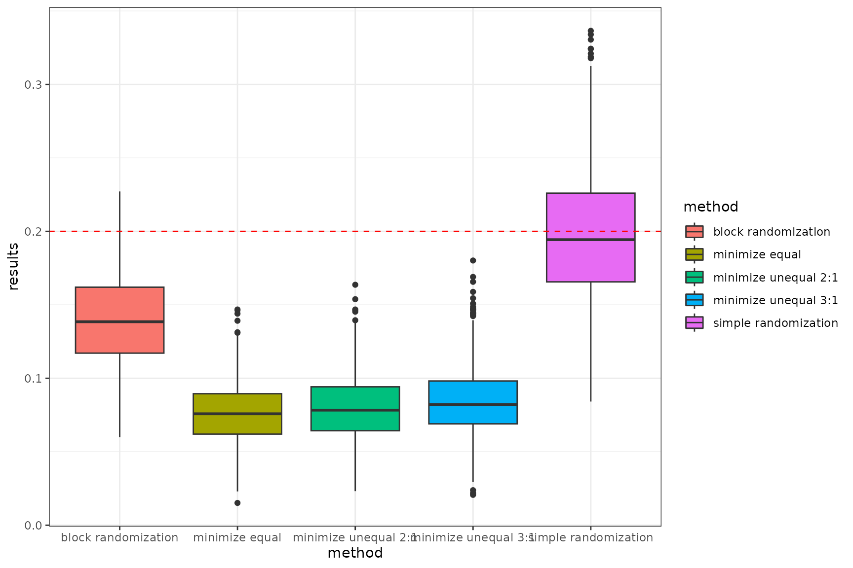
Summary average smd in each randomization methods
- Violin plot
# violin plot
cov_balance_data |>
  ggplot(aes(x = method, y = results, fill = method)) +
  geom_violin() +
  geom_hline(
    yintercept = 0.2,
    linetype = "dashed",
    color = "red"
  ) +
  facet_wrap(~covariants, ncol = 3) +
  theme_bw() +
  theme(axis.text = element_text(angle = 45, vjust = 0.5, hjust = 1))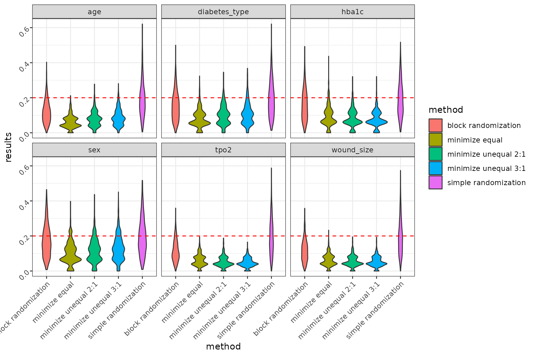
Summary smd in each randomization methods in each covariants
- Summary table of success
Based on the specified precision threshold of 0.2, a function
defining randomization success, named success_power, was
developed. If the SMD test value for each covariate in a given iteration
is above 0.2, the function defines the analysis data as ‘failure’ - 0;
otherwise, it is defined as ‘success’ - 1.
The final success power is calculated as the sum of successes in each iteration divided by the total number of specified iterations.
The results are summarized in a table as the percentage of success for each randomization method.
# function defining success of randomisation
success_power <-
  function(cov_data) {
    result_table <-
      lapply(unique(cov_data$simnr), function(i) {
        current_data <- cov_data[cov_data$simnr == i, ]

        current_data |>
          group_by(method) |>
          summarise(success = ifelse(any(results > 0.2), 0, 1)) |>
          tibble::add_column(simnr = i, .before = 1)
      }) |>
      bind_rows()

    success <-
      result_table |>
      group_by(method) |>
      summarise(results_power = sum(success) / n() * 100)

    return(success)
  }
success_power(cov_balance_data) |>
  as.data.frame() |>
  rename(`power results [%]` = results_power) |>
gt()| method | power results [%] |
|---|---|
| block randomization | 23.3 |
| minimize equal | 86.5 |
| minimize unequal 2:1 | 83.6 |
| minimize unequal 3:1 | 73.4 |
| simple randomization | 3.2 |
Conclusion
Considering all three randomization methods: minimization, block randomization, and simple randomization, minimization performs the best in terms of covariate balance. Simple randomization has a significant drawback, as patient allocation to arms occurs randomly with equal probability. This leads to an imbalance in both the number of patients and covariate balance, which is also random. This is particularly the case with small samples. Balancing the number of patients is possible for larger samples for n > 200.
On the other hand, block randomization performs very well in balancing the number of patients in groups in a specified allocation ratio. However, compared to adaptive randomisation using the minimisation method, block randomisation has a lower probability in terms of balancing the co-variables.
Minimization method, provides the highest success power by ensuring balance across covariates between groups. This is made possible by an appropriate algorithm implemented as part of minimisation randomisation. When assigning the next patient to a group, the method examines the total imbalance and then assigns the patient to the appropriate study group with a specified probability to balance the sample in terms of size, and covariates.